<Basis, Span, Change of Basis>
1. Install Packages
2. Basis
3. Span
4. Linear Combination, change of Basis
5. Inverse Matrix
Install Packages
필요한 Package 설치 및 import
# visualization을 위한 helper code입니다.
from urllib.request import urlretrieve
URL = 'https://go.gwu.edu/engcomp4plot'
urlretrieve(URL, 'plot_helper.py')

import sys
sys.path.append('../scripts/')

# 다음 세 custom function (1)plot_vector, (2)plot_linear_transformation, (3) plot_linear_transformations
# 을 사용할 것입니다.
from plot_helper import *
import matplotlib.pyplot as plt
import numpy as np
from mpl_toolkits.mplot3d import Axes3D
import scipy as sp
import scipy.linalg
import sympy as sy
sy.init_printing()
np.set_printoptions(precision=3)
np.set_printoptions(suppress=True)Basis
2차원 공간에서의 Basis
임의의 Horizontal Vector 및 Vertical Vector는 상수배해서 표현할 수 있다.
여기서, Horizontal Vector(1, 0), Horizontal Vector(0, 1)을 각각 i, j라고 할 시,
(편의상 Horizontal Vector는 (a, b)로 작성!)
2차원 공간에 있는 모든 Vector들은 Horizontal Vector + Vertical Vector의 합으로 표현이 가능하기 때문에
2차원 공간에 있는 모든 Vector들은 i와 j의 Linear Combination으로 나타낼 수 있다.
따라서, i와 j는 2차원 공간의 Basis Vector이다.

# Note
'''
아래의 plot_vector() 함수는 두 인자를 받습니다: (1) list of vectors, (2) list of tails (optional)
tails를 지정하지 않을 시 자연스럽게 tail은 origin으로 지정됩니다.
'''
# 예시

vectors = [(2,2)]
tails = [(-3,-2), (-3,1), (0,0), (1,-3)]
plot_vector(vectors, tails)
pyplot.title("The same vector, with its tail at four locations.");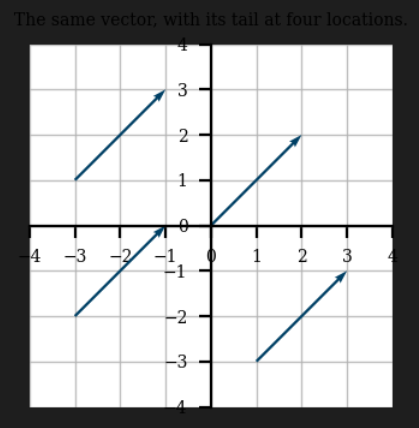
# basis vector
i = np.array((1,0))
j = np.array((0,1))

vec = 3*i + 2*j
vectors = [i, j, 3*i, 2*j, vec]
plot_vector(vectors)
pyplot.title("The vector $(3,2)$ as a linear combination of the basis vectors.");
Span
2차원 공간의 모든 Vector가 Basis의 Linear Combination으로 만들 수 있다.
→ i, j의 Span이 R2가 된다.
from numpy.random import randint
# span
vectors = []
i = numpy.array((1,0))
j = numpy.array((0,1))

for _ in range(1000):
    m = randint(-10,10)
    n = randint(-10,10)
    vectors.append(m*i + n*j)  # i, j (basis vecor)의 linear combination

plot_vector(vectors)
pyplot.title("1000 random vectors, created from the basis vectors");
이를 무수히 많은 Vector를 생성하면 R2공간을 전부 채울 수 있다.
만약 i, j가 아닌 (-2, 1), (1, -3)을 사용하면
# TODO:
# span
vectors = []
i = numpy.array((-2,1))
j = numpy.array((1,-3))

for _ in range(1000):
    m = randint(-10,10)
    n = randint(-10,10)
    vectors.append(m*i + n*j)  # i, j (basis vecor)의 linear combination

plot_vector(vectors)
pyplot.title("1000 random vectors, created from [-2,1], [1,-3]");
(-2, 1)과 (1, -3)을 사용해도 무수히 많은 vector를 사용하면 Linear Combination을 Plot할 시 R2를 전부 채울 수 있다.
→ Basis Vector로 반드시 i, j를 사용할 필요는 없다.
- Basis Vector로 i, j를 사용할 경우 vs. (-2, 1), (1, -3)을 사용할 경우
→ 계수(좌표)의 차이 발생
(-2, 1), (-1, 0.5)의 두 Vector를 Span:
# TODO:
# span
vectors = []
i = numpy.array((-2,1))
j = numpy.array((-1,0.5))

for _ in range(1000):
    m = randint(-10,10)
    n = randint(-10,10)
    vectors.append(m*i + n*j)  # i, j (basis vecor)의 linear combination

plot_vector(vectors)
pyplot.title("1000 random vectors, created from [-2, 1], [-1, 0.5]");
두 Vector (-2, 1), (-1, 0.5)가 Linearly Dependent하기 때문에
두 Vector의 Linear Combination으론 2차원 공간을 전부 채울 수 없다.
따라서, (-2, 1), (-1, 0.5)는 R2의 Basis가 될 수 없다.
Basis의 조건
- Basis는 해당 Subspace를 Span해야 한다.
- Basis를 Linear Combination해서 해당 Subspace의 어떤 Vector라도 만들 수 있어야 한다.
- Basis를 이루는 Vector들은 서로 Linearly Independent 해야한다.
두 Vector (3, 1, 0), (2, 0, 1)를 Linear Combination 했을 때:
fig = plt.figure(figsize = (8, 8))
ax = fig.add_subplot(projection='3d')

x2 = np.linspace(-2, 2, 10)
x3 = np.linspace(-2, 2, 10)
X2, X3 = np.meshgrid(x2, x3)
X1 = 3*X2 + 2*X3
ax.plot_wireframe(X1, X2, X3, linewidth = 1.5, color = 'g', alpha = .6)

vec = np.array([[[0, 0, 0, 3, 1, 0]],
               [[0, 0, 0, 2, 0, 1]],
               [[0, 0, 0, 10, 2, -2]]])
colors = ['r', 'b', 'purple']
for i in range(vec.shape[0]):
    X, Y, Z, U, V, W = zip(*vec[i,:,:])
    ax.quiver(X, Y, Z, U, V, W, length=1, normalize=False, color = colors[i],
              arrow_length_ratio = .08, pivot = 'tail',
              linestyles = 'solid',linewidths = 3, alpha = .6)

################################Dashed Line################################

point12 = np.array([[2, 0, 1],[5, 1, 1]])
ax.plot(point12[:,0], point12[:,1], point12[:,2], lw =3, ls = '--', color = 'black', alpha=0.5)

point34 = np.array([[3, 1, 0], [5, 1, 1]])
ax.plot(point34[:,0], point34[:,1], point34[:,2], lw =3, ls = '--', color = 'black', alpha=0.5)

#################################Texts#######################################
ax.text(x = 3, y = 1, z = 0, s='$(3, 1, 0)$', color = 'red', size = 16)
ax.text(x = 2, y = 0, z = 1, s='$(2, 0, 1)$', color = 'blue', size = 16)
ax.text(x = 10, y = 2, z = -2.3, s='$v (10,2,-2))$', color = 'purple', size = 16)

ax.set_xlabel('x-axis', size = 18)
ax.set_ylabel('y-axis', size = 18)
ax.set_zlabel('z-axis', size = 18)

ax.view_init(elev=-29, azim=130)
정의에 의해, 초록 Subspace의 Dimension = Subspace의 Basis의 개수
두 Vector의 Linear Independent 여부:
A = np.array([[3,2],[1,0],[0,1]])
np.linalg.matrix_rank(A)
→ A의 Rank가 2이므로 두 Vector는 서로 Linear Independent하다.
따라서, 두 Vector의 Basis의 두 조건을 모두 만족하기 때문에 초랙색 Subspace의 Basis가 된다.
→ 초록 Subspace는 전체 R3 공간 안에 속해있는, 2 Dimension의 Subspace (2차원 평면)가 된다.
위 그림의 v = (10, 2, -2)는 초록색 Subspace 바깥에 위치한다.
→ Ax = v의 해는 존재하지 않는다.
from sympy.solvers.solveset import linsolve

x1, x2 = sy.symbols('x1 x2')
A = sy.Matrix(((3,2),(1,0),(0,1)))
b = sy.Matrix((10,2,-2))
system = A,b
linsolve(system, x1, x2)
Linear Combination, change of Basis

(-2, 1), (1, -3)를 각각 a, b로 표현하면,
- {a, b} 를 Basis로 사용한 경우, (-7, 11)은 이 Basis의 계수가 (2, -3) 인 경우로 표현할 수 있다.
- {i, j}를 Basis로 사용할 경우, (-7, 11)은 이 Basis의 계수가 좌표 (-7, 11)인 경우로 표현할 수 있다.
(2, -3), (-7, 11)을 각각 c, c_라고 하면
- (-7, 11)은 Basis {a, b}에서 좌표 c(=(2, -3))으로 표현된다.
- (-7, 11)은 Basis {i, j}에서 좌표 c_(=(-7, 11))으로 표현된다.

즉 Matrix A = [[-2, 1], [1, -3]]에 Basis {a, b}의 좌표 c를 곱하면, basis {i, j}의 좌표 c_를 얻을 수 있다.
A = np.array([[-2,1],[1,-3]])
c = np.array([2,-3])
c_ = np.array([-7,11])

A
A@c
A에 i, j를 각각 곱하면,
i = np.array([1,0])
j = np.array([0,1])
A@i
A@j
→ Matrix A = [[-2, 1], [1, -3]]에 i를 곱했을 경우 a가 나오고 j를 곱했을 경우 b가 나온다.
plot_linear_transformation(A)
→ Linear Transformation은 원점 (0, 0)은 그 자리에 둔 채, 직선들(좌측 그림)을 다른 직선들(우측 그림)으로 Transform 한다.
A에 i(좌측 초록색 vector)를 곱했을 경우 a(우측 초록색 vector)가 나오고
A에 j(좌측 빨간색 vector)를 곱했을 경우 b(좌측 빨간색 vector)가 나온다.
즉, A (= [[-2, 1], [1, -3]]) 라는 Matrix는 Linear Transformation
→ Basis{a, b}를 Basis{i, j}로 바꾸는 Matrix
따라서,
Before Transformation의 Plot = Basis {a, b}
After Transformation의 Plot = Basis {i, j}
Square Matrix A: R(nxn)을 바라보는 2가지 방법
- Linear Transformation: Basis를 fix 시켜놓고, 해당 Basis에서 vector x1가 vector x2로 Linearly Transform되는 것을 행렬 A로 표현
- change of Basis: 같은 vector x는 Basis를 어떻게 잡냐에 따라 좌표가 달라진다.
Inverse Matrix
M = numpy.array([[1,2], [2,1]])
M_inv = inv(M)
# plot_linear_tranformation"s" 함수는 첫번째 인자, 두번째 인자를 차례대로 적용시켜줍니다.
plot_linear_transformations(M, M_inv)
Inverse M은 M에 의해 Linearly Transform된 직선들을 전부 원래 위치로 되돌려 놓는 Linear Transformation이라고 볼 수 있다.
→ (Inverse M)*M = I (Identity Matrix)
'Mathematics > Linear Algebra' 카테고리의 다른 글
| Advanced Eigendecomposition (0) | 2022.05.12 |
|---|---|
| Eigendecomposition (0) | 2022.05.11 |
| Gram-Schmidt orthonormalization & QR decomposition (0) | 2022.05.09 |
| Determinant, Least Square (0) | 2022.05.04 |
| Linear System, Inverse Matrix, Linear Combination (0) | 2022.05.02 |


